Your cart is currently empty!
Category: Cloud Data Engineering & Analytics
Scale your data architecture with cloud data engineering and analytics solutions that deliver flexibility, security, and cost‑efficiency. Explore how leading cloud platforms like AWS, Azure, and Google Cloud streamline data ingestion, storage, and transformation at petabyte scale. From building serverless pipelines and data lakes to implementing real‑time streaming analytics, our articles cover emerging trends like lakehouses, data mesh patterns, and AI‑powered data governance. Gain hands‑on tips for optimizing performance, ensuring compliance, and reducing total cost of ownership. Whether you’re migrating legacy warehouses or architecting greenfield cloud solutions, you’ll find everything you need here. Leverage the cloud—dive into Data Engineering & Analytics today!
-
What Is AWS Data Pipeline? Architecture, Use Cases & Modern Alternatives (2026 Guide)
AWS Data Pipeline is a managed web service from Amazon Web Services that automates the movement and transformation of data between different AWS services and on-premises data sources. It lets you define data-driven workflows where tasks run on a schedule and depend on the successful completion of previous tasks — essentially an orchestration layer for ETL (Extract, Transform, Load) jobs across your AWS infrastructure.
However, there is one critical update every developer and data engineer should know: AWS Data Pipeline is now deprecated. The service is in maintenance mode and is no longer available to new customers. In this guide, we cover everything about AWS Data Pipeline — how it works, its components, pricing, real-world use cases — and, most importantly, how to build a modern serverless data pipeline using EMR Serverless, SageMaker Pipelines, Lambda, SQS, and the Medallion Architecture on S3.
What Is AWS Data Pipeline?
AWS Data Pipeline is a cloud-based data workflow orchestration service that was designed to help businesses reliably process and move data at specified intervals. Think of it as a scheduling and execution engine for your data tasks.
At its core, AWS Data Pipeline allows you to:
- Move data between AWS services like Amazon S3, Amazon RDS, Amazon DynamoDB, and Amazon Redshift
- Transform data using compute resources like Amazon EC2 or Amazon EMR
- Schedule workflows to run at defined intervals (hourly, daily, weekly)
- Handle failures automatically with built-in retry logic and failure notifications
- Connect on-premises data sources with AWS cloud storage
The service was originally built to solve a common problem: data sits in different places (databases, file systems, data warehouses), and businesses need to move and transform that data regularly without writing custom scripts for every workflow.
Important: AWS Data Pipeline Is Now Deprecated
As of 2024, AWS Data Pipeline is no longer available to new customers. Amazon has placed the service in maintenance mode, which means:
- No new features are being developed
- No new AWS regions will be added
- Existing customers can continue using the service
- AWS recommends migrating to newer services
This is a significant development that affects any organization currently evaluating data orchestration tools on AWS. If you are starting a new project, you should skip AWS Data Pipeline entirely and choose one of the modern alternatives we cover later in this article.
For existing users, AWS has published migration guides to help transition workloads to services like Amazon MWAA (Managed Workflows for Apache Airflow) and AWS Step Functions.
How AWS Data Pipeline Works
AWS Data Pipeline operates on a simple but powerful execution model:
- You define a pipeline — a JSON-based configuration that specifies what data to move, where to move it, and what transformations to apply
- AWS Data Pipeline creates resources — it provisions EC2 instances or EMR clusters to execute your tasks
- Task Runner polls for work — a lightweight agent installed on compute resources checks for scheduled tasks
- Tasks execute — data is read from source, transformed, and written to the destination
- Pipeline monitors itself — built-in retry logic handles transient failures, and SNS notifications alert you to persistent problems
The execution follows a dependency graph. If Task B depends on Task A completing successfully, AWS Data Pipeline enforces that ordering automatically.
Scheduling Model
AWS Data Pipeline uses a time-based scheduling model. You define a schedule (for example, “run every day at 2 AM UTC”), and the pipeline creates a new execution instance for each scheduled run. Each instance processes data independently, making it easy to track success or failure for specific time windows.
Key Components of AWS Data Pipeline
Understanding the core components is essential to grasping how AWS Data Pipeline works:
Pipeline Definition
The pipeline definition is the blueprint of your data workflow. It is a JSON document that describes all the objects in your pipeline — data sources, destinations, activities, schedules, and their relationships.
Data Nodes
Data nodes define where your data lives — both the input source and the output destination:
- S3DataNode — Amazon S3 buckets and prefixes
- SqlDataNode — relational databases (RDS, EC2-hosted databases)
- DynamoDBDataNode — Amazon DynamoDB tables
- RedshiftDataNode — Amazon Redshift clusters
Activities
Activities define the work your pipeline performs:
- CopyActivity — moves data from one location to another
- EmrActivity — runs processing jobs on Amazon EMR clusters
- ShellCommandActivity — executes custom shell scripts on EC2 instances
- SqlActivity — runs SQL queries against databases
- HiveActivity — runs Apache Hive queries on EMR
Task Runners
Task Runners are lightweight agents that poll AWS Data Pipeline for scheduled tasks. When a task is ready, the Task Runner executes it on the assigned compute resource.
Preconditions
Preconditions are checks that must pass before a pipeline activity executes. For example, you might verify a source file exists in S3 before attempting to process it.
Schedules
Schedules define when your pipeline runs. You configure the start time, frequency, and end time. AWS Data Pipeline supports both one-time and recurring schedules.
AWS Data Pipeline Use Cases (Real-World Examples)
Before its deprecation, AWS Data Pipeline was commonly used for these scenarios:
1. E-Commerce Daily Sales ETL
Scenario: An online retailer needs to analyze sales performance across product categories and regions.
Every night at 2 AM, the pipeline extracts order data from their production RDS database, joins it with the product catalog stored in DynamoDB, aggregates sales by category and region, and loads the summary into Amazon Redshift.
Pipeline flow:
RDS → EC2 (transform & join) → RedshiftBusiness value: The marketing team opens their dashboard every morning and sees yesterday’s revenue breakdown by category, top-selling products, and regional performance — all without a single manual SQL query.
2. Web Server Log Processing & Analytics
Scenario: A SaaS company with 50 EC2 instances running Nginx wants to understand their traffic patterns.
The pipeline collects access logs from all instances daily, archives them to S3, and runs a weekly EMR job that processes the logs to generate reports: top pages by traffic, error rate trends, geographic distribution, and peak usage hours.
Pipeline flow:
EC2 logs → S3 (daily archive) → EMR (weekly analysis) → S3 (reports)Business value: The engineering team spots a 3x increase in 404 errors from mobile users, leading them to discover and fix a broken API endpoint that was costing them 12% of mobile traffic.
3. Healthcare Data Synchronization
Scenario: A hospital network runs their patient management system on an on-premises SQL Server database but wants their analytics team to work in AWS.
Every 6 hours, the pipeline syncs patient appointment data from the on-premises database to AWS RDS using the Task Runner installed on a local server. The data then feeds into Redshift for operational analytics.
Pipeline flow:
On-premises SQL Server → Task Runner → RDS → RedshiftBusiness value: Compliance-friendly data movement with full audit trails. The analytics team can predict patient no-show rates and optimize scheduling without touching the production database.
4. Financial Reporting Pipeline
Scenario: A fintech company must generate regulatory reports every quarter, which requires combining transaction data with compliance rules.
The pipeline extracts transaction records from DynamoDB, runs them through an EMR cluster that applies PII masking (replacing real names with hashes), converts currencies to USD, validates against compliance rules, and loads the clean dataset into Redshift.
Pipeline flow:
DynamoDB → EMR (PII masking + currency conversion) → RedshiftBusiness value: What used to take a compliance team 2 weeks of manual work now runs automatically in 4 hours, with consistent results every quarter.
5. Cross-Region Data Replication
Scenario: A global company with teams in the US and EU needs both teams to have access to fresh analytics data, but running cross-region queries is too slow and expensive.
The pipeline replicates the daily S3 data from
us-east-1toeu-west-1on a nightly schedule, so the European team queries local data with low latency.Pipeline flow:
S3 (us-east-1) → S3 (eu-west-1)Business value: EU analysts get sub-second query times instead of 30-second cross-region queries, and data transfer costs are predictable since it runs on a fixed schedule rather than on-demand.
AWS Data Pipeline Pricing
AWS Data Pipeline pricing is based on how frequently your activities run:
Activity Type Cost Low-frequency activity (runs once per day or less) $0.60 per activity per month High-frequency activity (runs more than once per day) $1.00 per activity per month Low-frequency precondition $0.60 per precondition per month High-frequency precondition $1.00 per precondition per month Free Tier
New AWS accounts (less than 12 months old) qualify for the AWS Free Tier:
- 3 low-frequency preconditions per month
- 5 low-frequency activities per month
Important: AWS Data Pipeline pricing covers only the orchestration. You still pay separately for the underlying compute (EC2 instances, EMR clusters) and storage (S3, RDS, Redshift) that your pipeline uses.
Pros and Cons of AWS Data Pipeline
Pros Cons Native AWS integration with S3, RDS, DynamoDB, Redshift, EMR Deprecated — no new features or region support Built-in retry and fault tolerance Dated UI and developer experience Supports on-premises data sources via Task Runner Limited to batch processing — no real-time support Schedule-based automation with dependency management Debugging failed jobs is difficult Low orchestration cost Lock-in to AWS ecosystem Visual pipeline designer in console JSON-based definitions are verbose and hard to maintain AWS Data Pipeline Alternatives (2026)
Since AWS Data Pipeline is deprecated, here are the recommended alternatives:
Amazon MWAA (Managed Workflows for Apache Airflow)
Amazon MWAA is the most direct replacement. It is a fully managed Apache Airflow service that handles the infrastructure for running Airflow workflows.
Best for: Complex, multi-step ETL workflows with branching logic and dynamic task generation.
AWS Step Functions
AWS Step Functions is a serverless orchestration service that coordinates AWS services using visual workflows.
Best for: Serverless architectures, event-driven processing, and workflows that integrate with Lambda functions.
Amazon EventBridge
Amazon EventBridge is an event bus that triggers workflows based on events from AWS services, SaaS applications, or custom sources.
Best for: Event-driven architectures where data processing starts in response to specific triggers.
Third-Party Alternatives
- Apache Airflow (self-hosted) — maximum flexibility, you manage the infrastructure
- Dagster — modern data orchestration with built-in data quality checks
- Prefect — Python-native workflow orchestration with a generous free tier
- dbt (data build tool) — focused on SQL transformations inside data warehouses
AWS Data Pipeline vs Step Functions
Feature AWS Data Pipeline AWS Step Functions Status Deprecated (maintenance mode) Actively developed Execution model Schedule-based Event-driven or schedule-based Compute EC2, EMR Lambda, ECS, any AWS service Serverless No (requires EC2/EMR) Yes (fully serverless) Pricing Per activity per month Per state transition Visual editor Basic Advanced (Workflow Studio) Error handling Retry with notifications Catch, retry, fallback states Real-time support No Yes For most new projects, AWS Step Functions is the better choice due to its serverless nature and active development.
Is AWS Data Pipeline Serverless?
No, AWS Data Pipeline is not serverless. It requires provisioning EC2 instances or EMR clusters to execute pipeline activities. The Task Runner agent must run on compute resources that you manage.
This is a key difference from modern alternatives like AWS Step Functions, which are fully serverless — you define your workflow, and AWS handles everything else.
Modern AWS Data Pipeline Architecture (2026)
Now that AWS Data Pipeline is deprecated, what does a modern data pipeline look like on AWS? Here is a production-ready architecture using current AWS services:
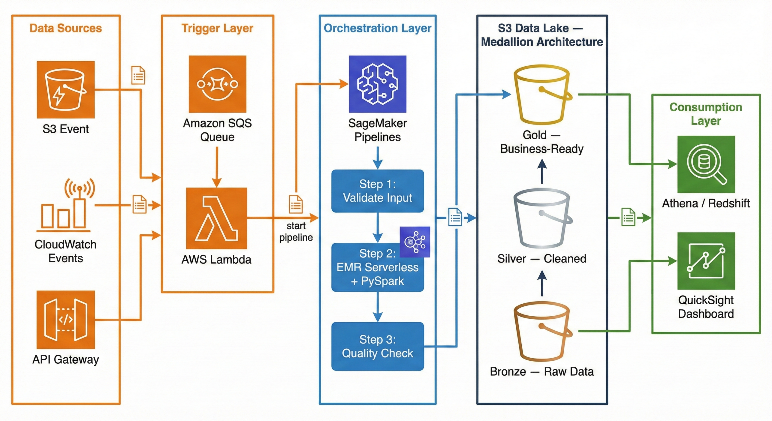
┌─────────────┐     ┌─────────────┐     ┌──────────────────────┐
│ Data Sources │     │  CloudWatch  │     │   API Gateway /      │
│  (S3 Event)  │────▶│  Events      │────▶│   External Triggers  │
└──────┬───────┘     └──────┬───────┘     └──────────┬───────────┘
       │                    │                        │
       ▼                    ▼                        ▼
┌──────────────────────────────────────────────────────────────┐
│                     Amazon SQS (Queue)                       │
│              Decouples triggers from processing              │
└──────────────────────────┬───────────────────────────────────┘
                           │
                           ▼
┌──────────────────────────────────────────────────────────────┐
│                    AWS Lambda (Trigger)                       │
│         Validates event, starts SageMaker Pipeline           │
└──────────────────────────┬───────────────────────────────────┘
                           │
                           ▼
┌──────────────────────────────────────────────────────────────┐
│              Amazon SageMaker Pipelines                      │
│                   (Orchestration)                             │
│                                                              │
│  ┌──────────┐   ┌───────────────┐   ┌────────────────────┐  │
│  │  Step 1:  │──▶│    Step 2:     │──▶│      Step 3:       │  │
│  │ Validate  │   │ EMR Serverless │   │  Quality Check     │  │
│  │  Input    │   │  + PySpark     │   │  + Write to Gold   │  │
│  └──────────┘   └───────────────┘   └────────────────────┘  │
└──────────────────────────────────────────────────────────────┘
                           │
                           ▼
┌──────────────────────────────────────────────────────────────┐
│                    Amazon S3 Data Lake                        │
│                                                              │
│  ┌────────────┐   ┌────────────┐   ┌─────────────────────┐  │
│  │   Bronze    │──▶│   Silver    │──▶│       Gold          │  │
│  │ (Raw Data)  │   │ (Cleaned)   │   │ (Business-Ready)   │  │
│  └────────────┘   └────────────┘   └─────────────────────┘  │
└──────────────────────────────────────────────────────────────┘
                           │
                    ┌──────┴──────┐
                    ▼             ▼
             ┌───────────┐  ┌──────────┐
             │ Redshift / │  │ QuickSight│
             │  Athena    │  │ Dashboard │
             └───────────┘  └──────────┘
Why This Architecture?
Trigger Layer — Lambda + SQS:
When a new file lands in S3 (or a scheduled CloudWatch Event fires), the event goes to an SQS queue. A Lambda function picks it up, validates the event, and kicks off the SageMaker Pipeline. Why SQS in between? It decouples the trigger from the processing. If the pipeline is busy, messages wait in the queue instead of being lost. If something fails, the message goes to a dead-letter queue for investigation.
Orchestration Layer — SageMaker Pipelines:
SageMaker Pipelines manages the end-to-end workflow. It defines each step as a node in a directed acyclic graph (DAG), handles retries, caches intermediate results, and provides a visual interface to monitor progress. While SageMaker is known for machine learning, its pipeline orchestration works perfectly for general-purpose data engineering too.
Processing Layer — EMR Serverless + PySpark:
Amazon EMR Serverless runs your PySpark jobs without you ever touching a cluster. You submit your Spark code, EMR Serverless provisions the exact resources needed, runs the job, and shuts down. You pay only for the compute time used. No cluster management, no idle costs, and it auto-scales based on your data volume.
Storage Layer — S3 Data Lake (Medallion Architecture):
Data flows through three layers in S3: Bronze (raw), Silver (cleaned), Gold (business-ready). This is called the Medallion Architecture, and we explain it in full detail in the next section.
Consumption Layer — Athena / Redshift + QuickSight:
Once data reaches the Gold layer, analysts query it using Amazon Athena (serverless SQL directly on S3) or Amazon Redshift (data warehouse). QuickSight dashboards visualize the results for business stakeholders.
Implementing Medallion Architecture on AWS: A Practical Guide
The Medallion Architecture is the most popular pattern for organizing data in a data lake. If you have ever struggled with messy, unreliable data, this pattern will make your life significantly easier.
What Is Medallion Architecture? (The Simple Explanation)
Think of it like a kitchen:
- Bronze = Raw groceries from the store. You bring them home and put them in the fridge exactly as they are — unwashed vegetables, sealed packages, everything in its original state. You don’t touch anything.
- Silver = Ingredients washed, chopped, and measured. You clean the vegetables, cut the meat, measure the spices. Everything is prepared and organized, but it is not a meal yet.
- Gold = The finished meal, plated and ready to serve. You have combined the prepared ingredients into a dish that anyone can eat and enjoy.
In data terms:
Layer What It Contains Who Uses It Bronze Raw data exactly as received from the source Data engineers (debugging, reprocessing) Silver Cleaned, validated, deduplicated data with enforced schema Data analysts, data scientists Gold Aggregated, business-ready tables optimized for dashboards Business users, executives, BI tools Why not just clean the data once and store it? Because requirements change. A business rule that seems right today might be wrong next month. By keeping the raw data in Bronze, you can always go back and reprocess it with new logic. You never lose the original truth.
S3 Folder Structure (How to Set It Up)
Here is the actual folder structure you would create in your S3 bucket. This is what a production data lake looks like:
s3://mycompany-data-lake/
│
├── bronze/
│   ├── orders/
│   │   ├── dt=2026-02-10/
│   │   │   └── orders_raw_001.json
│   │   ├── dt=2026-02-11/
│   │   │   └── orders_raw_001.json
│   │   └── dt=2026-02-12/
│   │       └── orders_raw_001.json
│   ├── customers/
│   │   └── dt=2026-02-12/
│   │       └── customers_export.csv
│   └── products/
│       └── dt=2026-02-12/
│           └── products_catalog.json
│
├── silver/
│   ├── orders/
│   │   └── dt=2026-02-12/
│   │       └── part-00000.snappy.parquet
│   ├── order_items/
│   │   └── dt=2026-02-12/
│   │       └── part-00000.snappy.parquet
│   ├── customers/
│   │   └── dt=2026-02-12/
│   │       └── part-00000.snappy.parquet
│   └── products/
│       └── dt=2026-02-12/
│           └── part-00000.snappy.parquet
│
└── gold/
    ├── fact_daily_sales/
    │   └── dt=2026-02-12/
    │       └── part-00000.snappy.parquet
    ├── dim_customer/
    │   └── part-00000.snappy.parquet
    ├── dim_product/
    │   └── part-00000.snappy.parquet
    └── dim_date/
        └── part-00000.snappy.parquet
Why this structure?
dt=YYYY-MM-DDpartitioning — Each date gets its own folder. This makes it trivial to reprocess a specific day or query a date range- Separate folders per data source —
orders/,customers/,products/are isolated. Each can have its own IAM access policy - Parquet files in Silver/Gold — Parquet is a columnar format that is 60-80% smaller than JSON and 10x faster to query
- JSON/CSV preserved in Bronze — We keep the original format so we always have the raw truth
Step-by-Step: Bronze Layer (Raw Data Landing)
The Bronze layer is the simplest. Your only job is to land the data exactly as received and tag it with when it arrived. No cleaning, no transforming, no filtering.
What happens at this stage:
- Raw data arrives from source systems (APIs, databases, file exports)
- You write it to S3 with a date partition
- You add metadata: ingestion timestamp, source system name, file name
E-commerce example: Your Shopify store sends a webhook with order data as JSON. You receive it and store it immediately.
# ============================================
# BRONZE LAYER: Ingest raw data — no changes
# ============================================
from pyspark.sql import SparkSession
from pyspark.sql.functions import current_timestamp, lit
from datetime import date

spark = SparkSession.builder \
    .appName("bronze-ingestion") \
    .getOrCreate()

today = date.today().isoformat()  # "2026-02-12"

# Read raw JSON from the source — could be an API export, S3 drop, etc.
raw_orders = spark.read.json("s3://source-bucket/shopify-exports/orders.json")

# Add metadata columns (when did we ingest this? from where?)
bronze_orders = raw_orders \
    .withColumn("_ingested_at", current_timestamp()) \
    .withColumn("_source_system", lit("shopify")) \
    .withColumn("_file_name", lit("orders.json"))

# Write to Bronze — append mode, never overwrite historical data
bronze_orders.write \
    .mode("append") \
    .json(f"s3://mycompany-data-lake/bronze/orders/dt={today}/")

print(f"Bronze: {bronze_orders.count()} raw orders ingested for {today}")
Key rules for Bronze:
- Never modify the data — store exactly what the source sends
- Always use append mode — never overwrite previous days’ data
- Add metadata —
_ingested_at,_source_system,_file_namehelp with debugging - Keep the original format — if the source sends JSON, store JSON
Step-by-Step: Silver Layer (Clean & Validate)
The Silver layer is where the real work begins. You take the messy Bronze data and turn it into something reliable and consistent.
What happens at this stage:
- Remove duplicate records
- Drop rows with missing critical fields
- Enforce data types (strings to dates, strings to decimals)
- Standardize formats (trim whitespace, normalize country names)
- Flatten nested structures (explode arrays into separate rows)
- Handle null values with sensible defaults
E-commerce example: The raw Shopify JSON has duplicate orders (webhooks sometimes fire twice), some orders have no
customer_id, prices are stored as strings, and email addresses have trailing spaces.# ================================================ # SILVER LAYER: Clean, validate, and standardize # ================================================ from pyspark.sql.functions import col, to_date, trim, when, explode from pyspark.sql.types import DecimalType # Read all Bronze data bronze_orders = spark.read.json("s3://mycompany-data-lake/bronze/orders/") print(f"Bronze records: {bronze_orders.count()}") # ---- STEP 1: Remove duplicates ---- # Shopify webhooks sometimes fire twice for the same order deduped = bronze_orders.dropDuplicates(["order_id"]) # ---- STEP 2: Drop invalid records ---- # Orders without order_id or customer_id are useless valid = deduped.filter( col("order_id").isNotNull() & col("customer_id").isNotNull() ) # ---- STEP 3: Enforce data types ---- typed = valid \ .withColumn("total_price", col("total_price").cast(DecimalType(10, 2))) \ .withColumn("order_date", to_date(col("created_at"))) # ---- STEP 4: Clean string fields ---- cleaned = typed \ .withColumn("email", trim(col("email"))) \ .withColumn("shipping_country", when(col("shipping_country").isNull(), "Unknown") .otherwise(trim(col("shipping_country"))) ) # ---- STEP 5: Write to Silver as Parquet ---- cleaned.write \ .mode("overwrite") \ .partitionBy("order_date") \ .parquet("s3://mycompany-data-lake/silver/orders/") removed = bronze_orders.count() - cleaned.count() print(f"Silver: {cleaned.count()} clean orders ({removed} bad records removed)")Flattening nested data (bonus):
Shopify orders contain a
line_itemsarray — each order has multiple products. In Bronze, this is stored as a nested array. In Silver, we explode it into separate rows:# Flatten line_items array into separate rows order_items = cleaned \ .select("order_id", "order_date", explode("line_items").alias("item")) \ .select( "order_id", "order_date", col("item.product_id").alias("product_id"), col("item.name").alias("product_name"), col("item.quantity").cast("int").alias("quantity"), col("item.price").cast(DecimalType(10, 2)).alias("unit_price") ) order_items.write \ .mode("overwrite") \ .partitionBy("order_date") \ .parquet("s3://mycompany-data-lake/silver/order_items/")Why Parquet? A 1GB JSON file becomes ~200MB in Parquet. Queries that used to take 30 seconds now take 3 seconds. Parquet stores data in columns, so when you query only
order_dateandtotal_price, it does not read the other 20 columns at all.Step-by-Step: Gold Layer (Business-Ready Aggregations)
The Gold layer is where data becomes useful for business decisions. You join tables, calculate KPIs, and build the datasets that power dashboards.
What happens at this stage:
- Join related tables (orders + products + customers)
- Aggregate data (daily totals, averages, counts)
- Calculate business metrics (revenue, average order value, conversion rates)
- Build fact and dimension tables (star schema)
E-commerce example: Build a daily sales summary that the marketing team can view in QuickSight.
# ================================================
# GOLD LAYER: Aggregate and build business tables
# ================================================
from pyspark.sql.functions import sum, count, avg, round, countDistinct

# Read cleaned data from Silver
orders = spark.read.parquet("s3://mycompany-data-lake/silver/orders/")
order_items = spark.read.parquet("s3://mycompany-data-lake/silver/order_items/")
products = spark.read.parquet("s3://mycompany-data-lake/silver/products/")

# Join order items with product details
enriched = order_items.join(products, "product_id", "left")

# Build daily sales summary
daily_sales = (
    enriched
    .groupBy("order_date", "category")
    .agg(
        round(sum(col("unit_price") * col("quantity")), 2).alias("total_revenue"),
        count("order_id").alias("total_items_sold"),
        countDistinct("order_id").alias("unique_orders"),
        round(avg(col("unit_price") * col("quantity")), 2).alias("avg_item_value")
    )
    .orderBy("order_date", "category")
)

# Write to Gold layer
daily_sales.write \
    .mode("overwrite") \
    .partitionBy("order_date") \
    .parquet("s3://mycompany-data-lake/gold/fact_daily_sales/")

daily_sales.show(5, truncate=False)
Sample output:
+----------+-------------+-------------+----------------+-------------+--------------+
|order_date|category     |total_revenue|total_items_sold|unique_orders|avg_item_value|
+----------+-------------+-------------+----------------+-------------+--------------+
|2026-02-12|Electronics  |45230.50     |312             |156          |145.00        |
|2026-02-12|Clothing     |12450.75     |178             |89           |69.95         |
|2026-02-12|Home & Garden|8920.00      |90              |45           |99.11         |
|2026-02-12|Books        |3240.00      |216             |108          |15.00         |
|2026-02-12|Sports       |6780.25      |67              |34           |101.20        |
+----------+-------------+-------------+----------------+-------------+--------------+
Now your marketing team can open QuickSight, filter by date and category, and see exactly how each product line performed — no SQL knowledge required.
Data Modeling at Each Layer
Each layer uses a different modeling approach. Here is why:
Layer Modeling Style What It Looks Like Why Bronze No model (source-as-is) Raw JSON from Shopify, CSV from CRM Preserve the original structure for auditing and reprocessing Silver Normalized (3NF-like) Separate orders,order_items,customers,productstables with foreign keysRemove redundancy, enforce data types, create an enterprise-wide clean dataset Gold Denormalized (Star Schema) Central fact_daily_salestable +dim_customer,dim_product,dim_dateFast queries, fewer joins, dashboard-ready Bronze Modeling
There is no modeling in Bronze. You store exactly what the source sends:
- Shopify sends nested JSON? Store nested JSON.
- CRM exports a CSV with 50 columns? Store the entire CSV.
- The only thing you add is metadata:
_ingested_at,_source_system,_file_name
Silver Modeling (Normalized)
In Silver, you create clean, separate tables with proper relationships:
silver_orders          silver_order_items       silver_customers       silver_products
─────────────          ──────────────────       ────────────────       ───────────────
order_id (PK)          order_item_id (PK)       customer_id (PK)       product_id (PK)
customer_id (FK) ───┐  order_id (FK) ──────┐    name                   name
order_date           │  product_id (FK) ─┐  │    email                  category
total_price          │  quantity         │  │    country                brand
email                │  unit_price       │  │    segment                price
shipping_country     │                   │  │    created_at             sku
status               │                   │  │
                     │                   │  │
                     └───────────────────┘  └── Relationships enforce
                                                data integrity
Key principle: Each piece of information is stored in exactly one place. A customer’s name exists only in
silver_customers, not duplicated across every order row.Gold Modeling (Star Schema)
The Gold layer uses a star schema — one central fact table surrounded by dimension tables, forming a star shape:
                    ┌──────────────┐
                    │  dim_date    │
                    │──────────────│
                    │ date         │
                    │ day_of_week  │
                    │ month        │
                    │ quarter      │
                    │ year         │
                    │ is_weekend   │
                    │ is_holiday   │
                    └──────┬───────┘
                           │
┌──────────────┐   ┌──────┴───────────┐   ┌──────────────┐
│ dim_customer │   │ fact_daily_sales │   │ dim_product  │
│──────────────│   │──────────────────│   │──────────────│
│ customer_id  │◄──│ order_date (FK)  │──▶│ product_id   │
│ name         │   │ customer_id (FK) │   │ name         │
│ segment      │   │ product_id (FK)  │   │ category     │
│ country      │   │ total_revenue    │   │ brand        │
│ lifetime_val │   │ total_orders     │   │ price_tier   │
└──────────────┘   │ avg_order_value  │   └──────────────┘
                   │ quantity_sold    │
                   └──────────────────┘
Why star schema for Gold?
When a business user asks “Show me total revenue by country for Q1 2026,” the query only needs to join
fact_daily_saleswithdim_customeranddim_date. That is 2 simple joins instead of scanning 5 normalized tables. BI tools like QuickSight, Power BI, and Tableau are specifically optimized for star schemas — they understand facts and dimensions natively.S3 Partitioning Strategy (How Data Is Partitioned)
Partitioning is how you organize files within each layer so that queries only read the data they need instead of scanning everything.
The Wrong Way (Avoid This)
Many tutorials teach the Hive-style
year/month/daypartitioning:s3://data-lake/bronze/orders/year=2026/month=02/day=12/Why this is a problem:
- Creates too many small partitions — each one triggers an S3 LIST API call
- Date range queries become complex:
WHERE year=2026 AND month=02 AND day>=10 AND day<=28 - Real-world teams have hit Athena query length limits when scanning 100+ days because the generated SQL is too long
- A query for “last 3 months” scans ~90 partitions with 3 API calls each = 270 API calls just for metadata
The Right Way (Use This)
Use a single date partition key in ISO 8601 format:
s3://data-lake/bronze/orders/dt=2026-02-12/Why this works better:
- Clean range queries:
WHERE dt BETWEEN '2026-02-01' AND '2026-02-28' - Natural alphabetical sorting (2026-01 comes before 2026-02)
- Each partition maps to exactly one date — no ambiguity
- Query engines prune efficiently on a single key
Partitioning Strategy by Layer
Layer Partition Key Example Path Why Bronze dt(ingestion date)bronze/orders/dt=2026-02-12/Track when data arrived from the source Silver dt(business event date)silver/orders/dt=2026-02-12/Query by when the business event happened Gold Business key + date gold/sales/region=US/dt=2026-02-12/Optimized for common dashboard filter patterns Partition Sizing Rule of Thumb
- Aim for 128MB to 1GB per partition file
- If your daily data is only 50MB, consider weekly partitions instead:
dt=2026-W07/ - Too many tiny files = slow queries (the “small file problem”)
- Too few giant files = slow writes and wasted memory
Storage Format by Layer
Layer Format Compression Size vs JSON Why Bronze JSON or CSV (as received) None or GZIP 1x (original) Preserve the exact source format Silver Apache Parquet Snappy ~0.2x (80% smaller) Columnar format, fast reads, great compression Gold Apache Parquet Snappy ~0.2x (80% smaller) Same benefits + optimized for Athena and Redshift Spectrum Best Practices for Medallion Architecture on AWS
# Best Practice Why It Matters 1 Never delete Bronze data You can always reprocess with new business rules 2 Use Parquet + Snappy in Silver/Gold 70-80% storage savings, 10x faster queries 3 Single-key date partitioning ( dt=YYYY-MM-DD)Simpler queries, better partition pruning 4 S3 Lifecycle policies — Bronze to Infrequent Access after 30 days, Glacier after 90 Cut storage costs by 50-70% for old data 5 Register tables in AWS Glue Data Catalog Athena, Redshift Spectrum, and EMR can all query by table name 6 Star schema in Gold BI tools are optimized for fact + dimension tables 7 Start with one data source Get orders working end-to-end before adding customers, products, etc. 8 Add metadata in Bronze ( _ingested_at,_source)Essential for debugging and data lineage How to Migrate from AWS Data Pipeline
If you are currently using AWS Data Pipeline and need to migrate:
- Audit your existing pipelines — document all pipeline definitions, schedules, data sources, and destinations
- Choose your target service — Amazon MWAA for complex ETL, Step Functions for serverless, SageMaker Pipelines for ML-integrated workflows
- Recreate pipeline logic — translate your pipeline definitions into the target format (Airflow DAGs, Step Functions state machines, etc.)
- Run in parallel — keep both old and new pipelines running to verify output consistency
- Validate data integrity — compare outputs from both systems
- Decommission — once confident, disable the AWS Data Pipeline version
Frequently Asked Questions
What is the difference between AWS Data Pipeline and ETL?
ETL (Extract, Transform, Load) is a process — it describes the pattern of pulling data from sources, transforming it, and loading it into a destination. AWS Data Pipeline is a tool that orchestrates ETL processes. The actual extraction, transformation, and loading are performed by other services like EMR, EC2, or Redshift.
Is AWS Data Pipeline still available?
For existing customers, yes — it continues to function. However, it is not available to new customers. AWS recommends Amazon MWAA or AWS Step Functions for new projects.
What replaced AWS Data Pipeline?
There is no single direct replacement:
- Amazon MWAA for complex ETL workflows (closest 1:1 replacement)
- AWS Step Functions for serverless orchestration
- SageMaker Pipelines for ML-integrated data workflows
- Amazon EventBridge for event-based triggers
Can I still use AWS Data Pipeline?
Yes, if you are an existing customer. However, you should start planning a migration since the service will not receive new features, and AWS could eventually announce an end-of-life date.
What is Medallion Architecture?
Medallion Architecture organizes data into three layers — Bronze (raw), Silver (cleaned), and Gold (business-ready). Each layer progressively improves data quality. It is the standard pattern for building data lakes on S3.
Is EMR Serverless better than regular EMR?
For most data pipeline use cases, yes. EMR Serverless eliminates cluster management — you submit your PySpark job and AWS handles provisioning, scaling, and termination. You pay only for the compute time used. Use regular EMR only if you need persistent clusters or custom configurations.
Conclusion
AWS Data Pipeline was a pioneering service that introduced many organizations to managed data orchestration on AWS. Its ability to schedule, execute, and monitor data workflows made it a valuable tool for batch processing and ETL automation.
However, with the service now in maintenance mode and unavailable to new customers, it is time to build with modern tools. The combination of SageMaker Pipelines for orchestration, EMR Serverless with PySpark for processing, Lambda + SQS for triggering, and the Medallion Architecture on S3 for storage gives you a production-ready, serverless, and cost-efficient data pipeline that scales from gigabytes to petabytes.
Whether you are building your first data pipeline or migrating from a legacy system, the key principles remain the same: keep your raw data safe in Bronze, clean it thoroughly in Silver, and serve it beautifully in Gold.
Need help building modern data pipelines on AWS? At Metosys, we specialize in ETL pipeline development, AWS data engineering with Glue and Redshift, and workflow automation with Apache Airflow. Our data engineers can help you migrate from legacy systems or build new pipelines from scratch. Get in touch to discuss your project.
Sources:
-
Sentry vs CloudWatch (2026): Complete Comparison for Error Tracking & Monitoring
Choosing between Sentry and Amazon CloudWatch comes down to one question: are you monitoring your application or your infrastructure?
Sentry is a developer-first error tracking tool that catches application-level bugs, crashes, and performance issues with detailed stack traces. CloudWatch is AWS’s native monitoring service that tracks infrastructure metrics, collects logs, and triggers alarms across your entire AWS environment.
The short answer: most production teams use both — Sentry for catching bugs and CloudWatch for watching infrastructure. But if you can only choose one, this guide will help you decide.
Quick Comparison Table
Feature Sentry Amazon CloudWatch Primary focus Application error tracking AWS infrastructure monitoring Error tracking Excellent — stack traces, breadcrumbs, grouping Basic — log pattern matching only Performance monitoring Transaction tracing, web vitals Metrics, custom dashboards Log management Limited (focused on errors) Comprehensive — CloudWatch Logs Alerting Issue-based alerts, Slack/PagerDuty/email Metric alarms, composite alarms, SNS Setup time ~10 minutes (install SDK) Already enabled for AWS services Language support 30+ languages and frameworks Language-agnostic (log-based) AWS integration Via SDK (works anywhere) Native — built into every AWS service Free tier 5K errors/month, 10K transactions 10 custom metrics, 10 alarms, 5GB logs Paid pricing From $26/month (Team plan) Pay-per-use (varies widely) Best for Developers debugging application bugs Ops teams monitoring AWS infrastructure What Is Sentry?
Sentry is an open-source application monitoring platform that specializes in real-time error tracking and performance monitoring. When your code throws an exception, Sentry captures it immediately with the full context: stack trace, user information, browser details, breadcrumbs (the sequence of events that led to the error), and the exact line of code that failed.
What makes Sentry different:
- Automatic error grouping — Sentry intelligently groups similar errors together instead of flooding you with 10,000 duplicate alerts. If the same
TypeErrorhits 500 users, you see one issue with a count of 500. - Stack traces with source code — You see the exact line of code that failed, including the values of local variables at the time of the crash.
- Breadcrumbs — A timeline showing what happened before the error: which API calls were made, which buttons the user clicked, which pages they visited.
- Release tracking — Deploy a new version and Sentry tells you which errors are new, which are fixed, and which regressed.
- Performance monitoring — Track slow transactions, database queries, and API calls. See where your application spends its time.
- Session replay — Watch a video-like reconstruction of what the user saw and did before the error occurred.
Languages and frameworks supported:
JavaScript, TypeScript, React, Next.js, Vue, Angular, Python, Django, Flask, Node.js, Express, Java, Spring, Go, Ruby, Rails, PHP, Laravel, .NET, Rust, Swift, Kotlin, Flutter, React Native, and more — over 30 platforms.
What Is Amazon CloudWatch?
Amazon CloudWatch is AWS’s built-in monitoring and observability service. It collects metrics, logs, and events from virtually every AWS service and provides dashboards, alarms, and automated responses.
What makes CloudWatch different:
- Native AWS integration — CloudWatch is built into AWS. Your EC2 instances, Lambda functions, RDS databases, and S3 buckets automatically send metrics to CloudWatch without installing anything.
- Infrastructure metrics — CPU utilization, memory usage, disk I/O, network traffic, request counts, latency — CloudWatch tracks all of this out of the box for AWS services.
- CloudWatch Logs — A centralized log management system. Application logs, VPC flow logs, Lambda execution logs, and CloudTrail audit logs all go to one place.
- CloudWatch Alarms — Set thresholds on any metric and trigger actions: send an SNS notification, auto-scale an instance group, or run a Lambda function.
- CloudWatch Logs Insights — A query language for searching and analyzing logs. Think of it as SQL for your log data.
- Application Signals — A newer feature that provides application performance monitoring (APM) with auto-instrumentation for Java, Python, and .NET applications.
Services that integrate natively:
EC2, Lambda, RDS, DynamoDB, S3, ECS, EKS, API Gateway, SQS, SNS, Kinesis, Step Functions, CloudFront, Elastic Load Balancing, and virtually every other AWS service.
Sentry vs CloudWatch: Detailed Comparison
Error Tracking
This is where the two tools diverge the most.
Sentry was built specifically for error tracking. When an unhandled exception occurs in your application:
- Sentry captures the full stack trace with source map support
- Groups it with similar errors automatically
- Shows you the exact line of code, the variable values, and the user’s session
- Provides breadcrumbs showing the 20 events that led to the crash
- Tracks which release introduced the error
CloudWatch approaches error tracking differently. It relies on log-based error detection:
- Your application writes errors to stdout/stderr or log files
- CloudWatch Logs collects those log lines
- You create metric filters that match patterns like
"ERROR"or"Exception" - CloudWatch counts occurrences and can trigger alarms
The difference: Sentry gives you “This
TypeError: Cannot read property 'id' of undefinedstarted in release v2.3.1, affects 342 users, happens on the checkout page, and here is the exact code.” CloudWatch gives you “Your application logged 47 lines containing the word ERROR in the last hour.”Winner: Sentry — by a wide margin for application error tracking.
Performance Monitoring
Sentry provides application-level performance monitoring:
- Transaction tracing — See how long each API request takes, broken down by database queries, external API calls, and rendering time
- Web vitals — Track Core Web Vitals (LCP, FID, CLS) that affect your Google search ranking
- Slow query detection — Identify database queries that take too long
- Custom spans — Instrument specific code paths to measure performance
CloudWatch provides infrastructure-level performance monitoring:
- Service metrics — CPU, memory, disk, network for EC2, RDS, Lambda duration, API Gateway latency
- Custom metrics — Push any numeric value from your application
- CloudWatch Application Signals — Newer APM feature with auto-instrumentation (limited language support)
- Container Insights — Monitoring for ECS and EKS clusters
Winner: Depends. Sentry wins for application performance (where in my code is it slow?). CloudWatch wins for infrastructure performance (is my server running out of memory?).
Log Management
Sentry is not a log management tool. It captures error events, not log streams. You can attach breadcrumbs and context to errors, but Sentry is not designed to store and search terabytes of application logs.
CloudWatch Logs is a full-featured log management service:
- Centralized collection from all AWS services
- CloudWatch Logs Insights for searching with a SQL-like query language
- Log retention policies (1 day to 10 years, or indefinite)
- Export to S3 for long-term archival
- Real-time log streaming with subscriptions
Winner: CloudWatch — it is a dedicated log management platform. Sentry does not compete in this category.
Alerting & Notifications
Sentry alerting is issue-based:
- Alert when a new error is detected
- Alert when an error exceeds a frequency threshold (e.g., more than 100 in 5 minutes)
- Alert when an error affects a specific number of users
- Integrations: Slack, PagerDuty, Opsgenie, email, webhooks, Jira, GitHub
CloudWatch alerting is metric-based:
- Alert when a metric crosses a threshold (e.g., CPU > 80% for 5 minutes)
- Composite alarms (combine multiple conditions)
- Actions: SNS notifications, Lambda functions, Auto Scaling, EC2 actions
- Anomaly detection (uses ML to detect unusual patterns)
Winner: Tie. They alert on fundamentally different things. Sentry alerts on application errors. CloudWatch alerts on infrastructure metrics. You likely need both.
Integration & Compatibility
Sentry works anywhere:
- Install via SDK in your application code
- Works on AWS, GCP, Azure, on-premises, or your laptop
- 30+ language SDKs with framework-specific integrations
- Source map upload for minified JavaScript
- GitHub and GitLab integration for linking errors to commits
CloudWatch is AWS-native:
- Automatic metric collection for all AWS services
- CloudWatch agent for custom metrics and logs from EC2
- Works with non-AWS environments via the agent, but that is not its strength
- Tightly integrated with IAM, SNS, Lambda, and Auto Scaling
Winner: Sentry for multi-cloud or non-AWS environments. CloudWatch for AWS-heavy architectures.
Pricing Comparison
Sentry Pricing
Plan Price Includes Developer (Free) $0/month 5K errors, 10K performance transactions, 1 user Team $26/month 50K errors, 100K transactions, unlimited users Business $80/month 50K errors, 100K transactions, advanced features Enterprise Custom Volume discounts, dedicated support Additional usage is billed per event. Sentry offers spike protection to prevent surprise bills from sudden traffic increases.
CloudWatch Pricing
CloudWatch uses pay-per-use pricing that can be complex:
Component Free Tier Paid Rate Custom metrics 10 metrics $0.30/metric/month Alarms 10 alarms $0.10/alarm/month Logs ingested 5 GB/month $0.50/GB Logs stored 5 GB/month $0.03/GB/month Logs Insights queries — $0.005/GB scanned Dashboard 3 dashboards $3/dashboard/month Real-world cost example: A medium-sized application with 20 custom metrics, 15 alarms, 50GB of logs/month, and 2 dashboards costs roughly $35-50/month on CloudWatch. That is comparable to Sentry’s Team plan.
Winner: Sentry for predictable pricing. CloudWatch can get expensive with high log volumes but is “free” if you only use basic AWS service metrics.
Ease of Setup
Sentry setup (~10 minutes):
# Install the SDK
npm install @sentry/nextjs

# Initialize in your app
npx @sentry/wizard@latest -i nextjs
That is it. Sentry auto-detects errors, captures stack traces, and starts sending data immediately. The wizard configures source maps, release tracking, and performance monitoring.
CloudWatch setup (already running):
If you are on AWS, CloudWatch is already collecting basic metrics for your services. No setup needed for default metrics. However, custom metrics, detailed monitoring, and log collection require additional configuration:
- Install the CloudWatch agent on EC2 instances
- Configure log groups and retention policies
- Create metric filters for error detection
- Build dashboards and alarms manually
Winner: Sentry for time-to-first-insight. CloudWatch for zero-config infrastructure metrics.
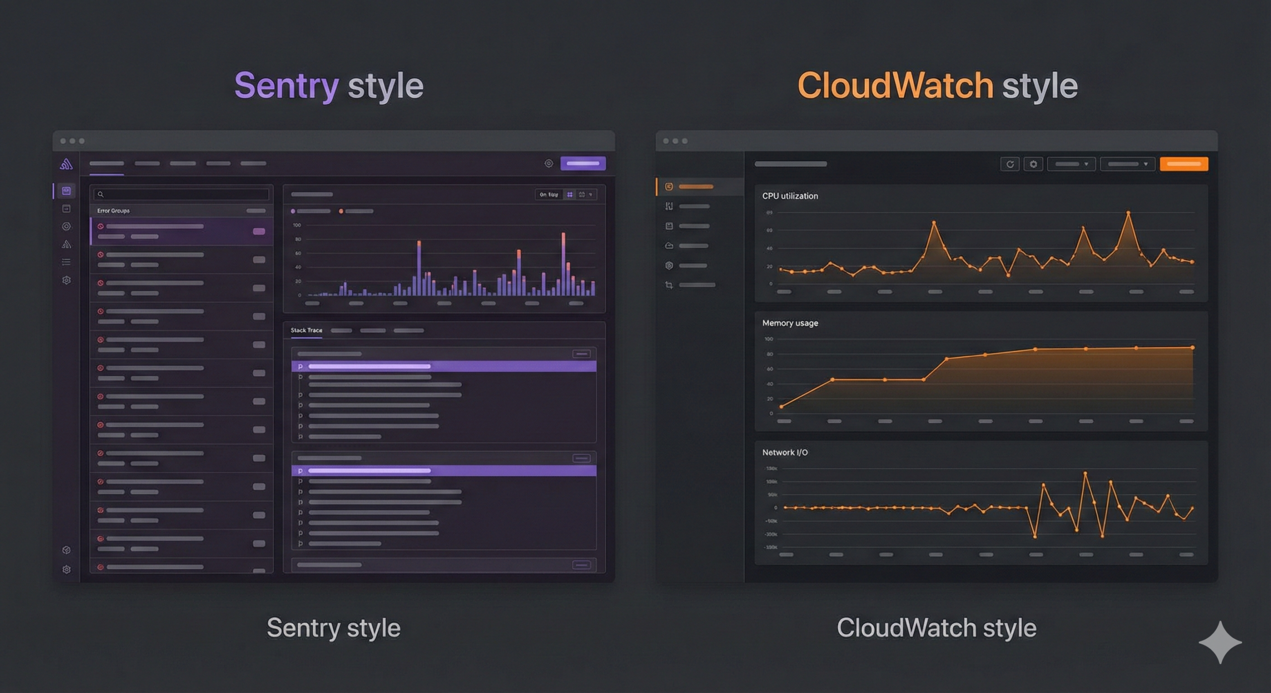
Dashboard & UI
Sentry has a modern, developer-focused UI:
- Issue list with real-time error counts and trend graphs
- Detailed error pages with stack traces, breadcrumbs, and user context
- Performance dashboards with transaction waterfall views
- Release health tracking with crash-free session rates
- Session replay viewer
CloudWatch has a functional but complex UI:
- Customizable metric dashboards with multiple widget types
- Logs Insights query editor with visualization
- Alarm management interface
- Application Signals dashboard (newer APM feature)
Winner: Sentry — the UI is designed for developers and is significantly more intuitive for debugging. CloudWatch’s UI is powerful but has a steeper learning curve.
When to Use Sentry
Choose Sentry when:
- You are a development team that needs to find and fix bugs fast
- You build web or mobile applications (React, Next.js, Python, Node.js, etc.)
- You want detailed error context — stack traces, breadcrumbs, session replay
- You need to track which release introduced a bug
- Core Web Vitals and frontend performance matter for your SEO
- You deploy to multiple cloud providers or on-premises
- You want to be up and running in under 15 minutes
Sentry is not ideal for: Infrastructure monitoring, server resource tracking, log aggregation, or AWS-specific operational metrics.
When to Use CloudWatch
Choose CloudWatch when:
- You are an ops or DevOps team managing AWS infrastructure
- You need to monitor server health — CPU, memory, disk, network
- You run serverless workloads on Lambda and want execution metrics
- You need centralized log management for compliance or auditing
- You want auto-scaling triggers based on real-time metrics
- Your entire stack is on AWS and you want native integration
- You want anomaly detection on infrastructure metrics
CloudWatch is not ideal for: Application-level error tracking, frontend performance monitoring, or debugging specific code issues.
Can You Use Both Together?
Yes — and most production teams do. Sentry and CloudWatch are complementary, not competing tools.
Here is how they work together:
Scenario CloudWatch Handles Sentry Handles Your API returns 500 errors Tracks the spike in 5xx metrics, triggers an alarm Captures the exact exception, stack trace, and affected users Lambda function times out Logs the timeout, tracks duration metrics Shows which code path caused the timeout and why Database connection pool exhausted Monitors RDS connection count, sends alarm Captures the ConnectionErrorwith the query that failedMemory leak in Node.js Tracks EC2 memory usage trending upward Captures OutOfMemoryErrorwith heap snapshot contextFrontend JavaScript crash Not applicable (CloudWatch is server-side) Captures the error with browser info, user session, and replay The workflow looks like this:
- CloudWatch alarm fires: “5xx error rate exceeded 5% on API Gateway”
- On-call engineer opens Sentry to see what is actually failing
- Sentry shows:
TypeError: Cannot read property 'items' of nullincheckout.js:142, started 20 minutes ago, affects 89 users, introduced in releasev3.2.1 - Engineer rolls back to
v3.2.0, Sentry confirms the error stopped
CloudWatch tells you something is wrong. Sentry tells you what, where, and why.
Sentry vs CloudWatch vs Datadog
Some teams also consider Datadog as an all-in-one alternative. Here is how it compares:
Feature Sentry CloudWatch Datadog Error tracking Excellent Basic Good Infrastructure monitoring None Excellent Excellent APM Good Basic (Application Signals) Excellent Log management Minimal Good Excellent Pricing Affordable ($26+/mo) Pay-per-use Expensive ($15+/host/mo) Setup complexity Low Low (on AWS) Medium Best for Dev teams AWS ops teams Enterprises wanting one tool When to choose Datadog: You want a single platform for infrastructure, APM, logs, and error tracking, and you have the budget. Datadog starts at $15/host/month for infrastructure monitoring, plus additional costs for APM, logs, and error tracking — which can add up quickly for larger deployments.
When to skip Datadog: You are a small-to-medium team and the cost is not justified. Sentry (errors) + CloudWatch (infrastructure) gives you 90% of Datadog’s value at a fraction of the cost.
Frequently Asked Questions
Is Sentry free?
Yes, Sentry offers a free Developer plan that includes 5,000 errors per month, 10,000 performance transactions, and 500 session replays. It is limited to one user, but it is a great way to try Sentry before upgrading. The Team plan starts at $26/month with unlimited users.
Can CloudWatch track application errors?
Sort of. CloudWatch can detect errors in logs using metric filters (matching patterns like “ERROR” or “Exception”), but it does not provide stack traces, error grouping, or debugging context. For true application error tracking, you need a dedicated tool like Sentry.
Is Sentry better than CloudWatch?
They serve different purposes. Sentry is better for application error tracking and debugging. CloudWatch is better for infrastructure monitoring and log management. Most teams use both. Comparing them directly is like comparing a debugger to a server dashboard — they solve different problems.
What is the best monitoring tool for AWS?
For a complete monitoring stack on AWS, we recommend:
- CloudWatch for infrastructure metrics and logs (it is already there)
- Sentry for application error tracking and performance monitoring
- CloudWatch Alarms + SNS for operational alerts
- Sentry Alerts for development/bug alerts
This combination covers infrastructure health, application errors, and performance monitoring without the cost of an all-in-one platform like Datadog.
Can I self-host Sentry?
Yes, Sentry is open-source and can be self-hosted. The self-hosted version is free and includes most features. However, self-hosting requires managing the infrastructure (PostgreSQL, Redis, Kafka, ClickHouse), which is a significant operational burden. Most teams find the hosted version more cost-effective.
Does Sentry affect my application’s performance?
Sentry’s SDK is designed to be lightweight. It adds minimal overhead (~1-5ms per request for performance monitoring). Error capture only runs when an exception occurs. You can configure sample rates to reduce the volume of performance data collected if needed.
Conclusion
Sentry and CloudWatch are not competitors — they are partners in a complete monitoring stack.
- Use CloudWatch to watch your AWS infrastructure: are your servers healthy, are your Lambda functions running, are your logs centralized?
- Use Sentry to watch your application code: are there bugs, which release caused them, which users are affected, and where exactly in the code did things go wrong?
If you are forced to choose one: pick CloudWatch if you are an ops-focused team running serverless workloads entirely on AWS. Pick Sentry if you are a development team shipping features fast and need to catch bugs before your users report them.
But the best answer? Use both. CloudWatch is already running if you are on AWS. Adding Sentry takes 10 minutes and immediately gives you superpowers for debugging production issues.
Need help setting up production-grade monitoring for your application? At Metosys, we specialize in monitoring with Sentry, Prometheus & CloudWatch and real-time metrics and reporting systems. We can design a monitoring stack that catches bugs before your users do. Get in touch to discuss your setup.
Sources:
- Automatic error grouping — Sentry intelligently groups similar errors together instead of flooding you with 10,000 duplicate alerts. If the same
-

Why Every Modern Application Needs a Digital Detective
Have you ever been navigating a critical application, and suddenly—POOF—it just stops working? Maybe the screen freezes, or a process fails silently in the background. These technical failures, or bugs, are like invisible friction points that crawl into the codebase and disrupt the user experience.
For developers, identifying the root cause of these issues in a production environment is like playing a game of Where’s Waldo?—except Waldo is invisible and hiding within millions of lines of distributed code. This is where Sentry comes into play.
In this comprehensive guide, we will explore why Sentry is considered the gold standard for error tracking, and we will compare it against industry heavyweights like AWS CloudWatch, Splunk, and Google Analytics. Whether you are managing a small startup or a global enterprise, choosing the right “digital detective” is critical for your 2025 technology roadmap.
Sentry Working: How the Digital Detective Pinpoints Errors
To understand sentry working, imagine your application as a complex machine. Every time a component fails or a calculation goes wrong, a specialized “watchdog” (Sentry) immediately records the state of the machine and alerts the maintenance team.
1. The Super-Secret SDK (The Monitor)
First, developers integrate a lightweight library into their application, known as an SDK. Think of this as giving your codebase a nervous system. This monitor doesn’t track private user behavior; it strictly watches the code execution. When the application encounters an unhandled exception, the SDK intercepts the data before the session ends.
2. The Information Payload (The Event)
When an error occurs, Sentry captures an “event.” This is similar to a detective collecting a detailed report from a crime scene. Inside this event, Sentry includes:
- The Stack Trace: A chronological map of every function call leading up to the crash.
- The Context: Metadata about the environment, such as browser version, OS, and release version.
- The Impact: Sentry quantifies how many unique users are affected by the issue.
3. The Centralized Dashboard
All captured events are sent to Sentry’s centralized platform. Rather than showing a raw list of logs, Sentry uses “fingerprinting” to group identical errors into single “Issues.” This prevents noise and allows developers to prioritize the most critical failures first.
By observing sentry working in real-time, engineering teams can shift from reactive firefighting to proactive resolution, fixing bugs before they spiral into system-wide outages.
Sentry vs AWS CloudWatch: The Specific Specialist vs. The General Guard
One of the most frequent debates in the DevOps world is sentry vs aws cloudwatch.
Imagine managing a high-rise skyscraper.
- AWS CloudWatch is the Building Security Team. They monitor the elevators, the HVAC systems, the electrical grid, and the external perimeter. They ensure the overall infrastructure (the skyscraper) is healthy.
- Sentry is the Internal Monitor focused on specific rooms. It doesn’t care about the elevators; it cares if a specific faucet is leaking or if a lightbulb in room 402 has burned out.
Sentry vs AWS CloudWatch: The Key Differences
When evaluating sentry vs aws cloudwatch, you are essentially choosing between infrastructure monitoring and application-level code monitoring.
- AWS CloudWatch excels at infrastructure health: “The server CPU is at 99%!” or “The database is running slow.”
- Sentry excels at code-level logic errors: “This specific function failed for users in the checkout flow.”
Modern enterprises typically use both. CloudWatch monitors the “host” (your AWS resources), while Sentry monitors the “guest” (your application code).
Sentry vs AWS: Platform vs. Tool
When discussing sentry vs aws, it’s important to remember that AWS is a vast cloud ecosystem offering hundreds of services. Sentry is a specialized, best-in-class tool for a single purpose: error management.
While AWS offers logging tools (CloudWatch Logs), they are often raw and require significant manual filtering. Sentry transforms that raw data into actionable intelligence, providing a developer experience that a general-purpose cloud provider struggles to match.
Sentry vs CloudWatch RUM: User Experience vs. Network Health
AWS offers a specialized feature called RUM (Real User Monitoring). When comparing sentry vs cloudwatch rum, it’s helpful to distinguish between how a user moves through your app and why their experience broke.
- CloudWatch RUM is like a satellite view. It tracks page load times, geographical latencies, and “User Journeys.” It tells you that a user in Berlin is experiencing slow performance.
- Sentry is like a BlackBox recorder. It doesn’t just see the slowness; it captures the specific function call or API timeout that caused it.
If your goal is to optimize the global speed of your website, CloudWatch RUM is an excellent choice. However, if your goal is to minimize time-to-fix for code regression, Sentry is the clear winner. In the sentry vs cloudwatch rum showdown, Sentry provides the “why” while RUM provides the “where.”
Sentry vs CloudWatch Reddit: The Developer Consensus
If you browse tech communities like Reddit, you will find heated discussions regarding sentry vs cloudwatch reddit.
A common sentiment on Reddit is that while CloudWatch is comprehensive, it is notoriously “noisy” and lacks a cohesive user interface (UI). One user might say, “I use CloudWatch because we are already on the AWS stack,” while another responds, “Sentry’s UI allows my team to solve in 5 minutes what took 2 hours in CloudWatch Logs.”
The community consensus on sentry vs cloudwatch reddit generally follows these three points:
- Setup Speed: Sentry is considered “plug-and-play,” whereas CloudWatch often requires complex IAM roles and log group configurations.
- Context: Sentry provides source-mapped stack traces out of the box; CloudWatch often leaves you staring at minified production logs.
- Alerting: CloudWatch alerts are great for infrastructure (e.g., “CPU high”), but Sentry alerts are actionable for developers (e.g., “Database timeout on line 42”).
Ultimately, the sentry vs cloudwatch reddit threads suggest a hybrid approach: Use CloudWatch for system health and Sentry for application-level observability.
Sentry vs Application Insights: Ecosystem Lock-in vs. Portability
For teams operating within the Microsoft ecosystem, the comparison is often sentry vs application insights.
- Application Insights (part of Azure Monitor) is deeply integrated with the .NET and Azure stack. It offers excellent “autodiscovery” for Microsoft services.
- Sentry is an agnostic detective. It works seamlessly across Azure, GCP, AWS, and on-premise environments.
The choice in sentry vs application insights often comes down to portability. If you ever plan to move part of your stack out of Azure, Sentry’s cross-platform nature ensures your observability doesn’t break. Furthermore, many developers find Sentry’s focus on “Issue grouping” to be superior to the raw telemetry viewing in Application Insights.
Sentry vs Splunk: Tactical Triage vs. Enterprise Auditing
Finally, let’s look at sentry vs splunk. This is a comparison between a scalpel and a chainsaw.
- Splunk is a “Data Giant.” It is designed to ingest massive volumes of machine data for security auditing, compliance, and historical analysis. It excels at answering retrospective questions: “Who accessed this file six months ago?”
- Sentry is an “Actionable Triage” tool. It doesn’t care about your historical login logs; it cares about the crash that is happening right now.
In the sentry vs splunk debate, companies often find that Splunk is too expensive and slow for simple error tracking. Sentry is built to help a developer fix a bug in minutes. Splunk is built to help a data analyst find patterns over weeks.
Sentry vs Google Analytics: Engagement vs. Stability
A prevalent misconception in the industry is that a website with traffic analytics doesn’t need error monitoring. This brings us to the sentry vs google analytics comparison.
Consider the operation of an E-commerce Platform.
- Google Analytics is your window into user behavior. It tracks conversion rates, referral sources, and popular products. It’s essential for understanding who your customers are and what they are doing.
- Sentry is your window into application stability. It monitors the “buy” button, the checkout API, and the payment gateway integration. It tells you why a customer cannot complete their purchase.
In the world of sentry vs google analytics, these tools are complementary. Google Analytics might report a high bounce rate on your checkout page, but without Sentry, you won’t know if users are leaving because the price is too high or because the checkout script is crashing.
Sentry Self Hosted Pricing: The Cost of Ownership vs. Convenience
For teams looking to optimize their budget, the question of cost is paramount. When researching sentry self hosted pricing, it is vital to look beyond the $0 price tag of the software license.
The Self-Hosted Reality (On-Premise)
Sentry is an open-source project, meaning you can host the core platform on your own infrastructure for free. However, “free” often refers to the license, not the total cost of ownership (TCO).
Key considerations for sentry self hosted pricing include:
- Infrastructure Costs: Sentry depends on multiple heavy-duty services (PostgreSQL, Clickhouse, Kafka, Redis). Running these reliably in the cloud typically costs between $50 and $250 per month in compute and storage.
- Maintenance Overhead: When you host Sentry, you are responsible for upgrades, security patches, and database scaling. This often requires several hours of DevOps time per month.
- Feature Gatekeeping: While Sentry maintains high parity between its SaaS and self-hosted versions, certain advanced AI features and mobile symbolication services are proprietary and exclusive to the SaaS offering.
Ultimately, the decision on sentry self hosted pricing depends on your team’s size. Small teams usually save money and time by using Sentry’s SaaS tier, while giant enterprises with existing Kubernetes clusters might find value in self-hosting.
Sentry Rate and Quotas: Managing Ingestion Flow
The final technical concept to master is the sentry rate. This refers to the volume of events your application sends to the monitoring platform.
In a high-traffic environment, a single recursive bug can trigger millions of errors in seconds. If your sentry rate is not managed properly, two things happen:
- Quota Exhaustion: You might hit your monthly plan limit within hours.
- Dashboard Noise: Your “Issues” list becomes impossible to parse due to the sheer volume of identical events.
Developers manage the sentry rate through “Sampling.” By setting a sample rate (e.g., 10%), Sentry only ingests one out of every ten events. This provides enough statistical data to identify patterns without blowing your budget or overwhelming your engineers.
Conclusion: Crafting Your Observability Strategy
We have covered a significant amount of ground, from comparing sentry vs cloudwatch rum to deconstructing the hidden costs of sentry self hosted pricing.
The most important takeaway is that observability is not a “one size fits all” solution. Leading engineering teams often adopt a multi-tool approach:
- AWS CloudWatch for infrastructure-level health.
- Google Analytics for product and marketing insights.
- Sentry for code-level stability and rapid bug resolution.
If you are just starting out, prioritize Sentry. Its developer-first approach and the transparency of its sentry working model make it the most effective tool for maintaining high application quality. By integrating Sentry today, you are not just tracking errors—you are investing in a better experience for your users.
Advanced Observability Strategies
Once you have mastered the basics of comparing sentry vs aws cloudwatch, you can begin implementing advanced strategies to further harden your application.
1. AI-Powered Root Cause Analysis
In 2025, Sentry introduced advanced AI capabilities that go beyond simple error reporting. The platform can now analyze a crash and suggest specific code fixes (Source Map awareness). This is a primary differentiator when evaluating sentry vs aws—while AWS provides the data, Sentry provides the answer.
2. Ecosystem Integration
A key advantage of Sentry is its ability to integrate with your existing developer workflow. By connecting Sentry to tools like Slack, Microsoft Teams, or GitHub, your engineering team receives real-time notifications about regressions. This reduces the “mean time to resolution” (MTTR) far more effectively than manually searching through logs in sentry vs splunk.
The Ultimate “Which Tool Should I Choose?” Checklist
Are you still confused? Don’t worry! Here is a simple checklist to help you decide which superhero tool belongs in your digital treehouse:
If your primary goal is to… Use this tool! Reason for selection Debug code-level production crashes Sentry Direct mapping to source code and line numbers. Monitor server CPU and infrastructure AWS CloudWatch Native integration with AWS resource health. Understand user interaction latencies CloudWatch RUM Excellent for tracking frontend performance metrics. Use the community-preferred tool Sentry High developer sentiment on Reddit for UI/UX. Standardize on the Microsoft stack Application Insights Frictionless integration with .NET/Azure. Perform deep security/compliance audits Splunk Unmatched capacity for massive log ingestion. Track marketing and user funnel data Google Analytics The industry standard for behavior analytics. Glossary of Key Terms
To solidify your understanding of sentry working and the broader observability landscape, keep this glossary handy:
- SDK (Software Development Kit): A lightweight library integrated into your code to monitor execution.
- Event: A single unit of data representing a crash, error, or performance transaction.
- SaaS (Software as a Service): A hosted model where Sentry manages the infrastructure for you.
- Self-Hosted: On-premise deployment where you manage the database and compute resources.
- Infrastructure: The underlying hardware and cloud services (AWS, Azure) that host your app.
- Log: A historical record of system events, often used for post-mortem analysis.
- Sampling: The process of capturing a percentage of data to manage costs and noise.
Final Thoughts: Building a Resilient Future
In 2025, the barrier between success and failure is often the speed at which a team can identify and resolve technical debt. By understanding the nuances of sentry vs cloudwatch rum, evaluating sentry self hosted pricing objectively, and acknowledging the strengths of sentry vs application insights, you are empowered to make a data-driven decision.
Start small, focus on the errors that impact your users most, and leverage the transparency of sentry working to build more reliable software.
-

Predicting Flight Delays with Machine Learning: How Fly Dubai Uses AI to Forecast On-Time Performance
1. Introduction: Turning Turbulence into Predictability
When a flight is delayed, it costs airlines a lot of money. The biggest loss is trust. For travelers, even a short delay can ruin their plans. To succeed, airlines must be reliable.
Imagine the challenge for an airline with hundreds of flights every day. Old systems cannot keep up when weather or traffic changes quickly. Most airlines react after delays happen. But what if they could predict them hours before?
That is where machine learning comes in. Airlines like FlyDubai use data to predict delays. They look at history and current conditions to forecast delays before the plane takes off. This gives the team time to fix issues with the crew or gates.
At the center of this is a smart computer system. This helps airlines learn from new data and make better predictions every day.
2. Understanding the Problem: One Delay Leads to Another
Every flight has two parts, leaving and arriving. These two are connected. If a plane is late going one way, it will likely be late coming back.
Let’s look at an example. A plane flying from Dubai to Karachi gets delayed because of bad weather. That same plane has to fly back to Dubai later. Because it arrived late, it will leave late again. This affects the next group of passengers and crew. It creates a chain of delays.
This is a big problem for airlines. One delay causes another. A late flight out means a late flight in. It becomes a loop.
Many things cause this:
- Weather issues like storms.
- Plane type and how long it takes to get ready.
- Crew hours because pilots can only work for so long.
- Busy airports where planes have to wait.
- Air traffic rules that limit flights.
Imagine hundreds of flights every day. You can see why it is hard to stop delays.
Airlines work in a world where data changes every minute. Weather updates and gate changes happen all the time. A computer model built on old data might be wrong today.
This creates another problem called model decay. Even a good model can become bad over time if the world changes. New flight paths or seasons make the old data less useful.
That is why airlines need a smart system. They need a system that learns on its own. It should know when things change and fix itself.
The goal isn’t just to predict one delay. It is about managing the whole system where everything is connected.
3. The ML Pipeline Architecture
In aviation, data moves very fast. We need to handle it well. First, we must answer: what is aws data pipeline? It is a service that helps move data easily. Fly Dubai uses scalable data pipelines to handle millions of data points. This helps them adapt to changes in real time.
Think of it as a digital twin of the airline. It is a living system where data flows smoothly. This is sometimes called a datapipe aws solution. It goes from getting data to making predictions without any manual work.
3.1 Data Ingestion:
Every journey begins with getting the data. Aws data pipeline helps here. The system pulls current and past data from many places like schedules, logs, and weather reports. You might ask, what is data pipeline in aws used for here? It connects all these data sources. The data is checked and stored in a data lakehouse. This makes sure everything is ready for the next steps.
3.2 Feature Engineering & Storage
Once we have the data, we need to make it useful. This step is called feature engineering. It turns raw numbers into helpful hints for the computer.
Some examples are:
- Average delay for a specific route.
- How long it takes to turn a plane around.
- How busy an airport is.
- How tired the crew might be.
All these hints are stored in a central place called a Feature Store. This keeps everything organized. It helps different computer models use the same information to learn.
3.3 Model Training
The heart of the system is where the learning happens. Instead of writing new code for every model, the team uses a configuration file options. This file tells the system what data to use and how to learn.
When new data comes in, the system starts learning automatically. It uses powerful cloud computers to build many models at once. For example:
- Yes or No models to guess if a flight will be delayed.
- Number models to guess how many minutes the delay will be.
The best models are saved and ready to be used.
3.4 Batch Inference
Every day, the system wakes up and starts predicting. It looks at the flight schedule for the day. It uses the best models to make a forecast for every flight.
The results are shown on a real time kpi dashboard. This helps the team see what is happening right away using tools like Power BI or Tableau. They can see:
- Which flights might be late.
- Where they need extra planes or crew.
- When to tell passengers about a delay.
This happens automatically. No one has to push a button. It gives the airline a clear view of the future.
3.5 Drift Detection & Continuous Retraining
A good system keeps learning. The world changes, and the data changes too. This is called drift.
The system watches for drift. It checks if the new data looks different from the old data. It uses math tests to find small differences.
If the data changes too much, the system knows it needs to learn again. It starts a new training session with the latest data. This keeps the predictions accurate even as things change.
3.6 A Flexible System
This system is built to be flexible. By using simple configuration files, it can handle many different jobs:
- Predicting flight delays.
- Planning crew schedules.
- Guessing when planes need repair.
- Understanding what passengers want.
A small change in the file can update the whole system. This makes it easy to maintain and ready for the future.
4. Data Transformation & Feature Engineering
Airlines create a lot of data every second. This includes departure times, aircraft numbers, and weather reports. Raw data is messy. It is like crude oil. It needs to be cleaned before we can use it. This process is called data transformation.
In Fly Dubai’s system, this step is very important. It turns messy data into clean information that helps predict delays.
4.1 The Pre-Flight Checklist: Data Transformation
Before the computer can learn, the data must be checked. This is like a pre-flight safety check.
Data comes from many places. Some timestamps are different. Some records are missing. The system fixes these problems automatically:
- It fixes time zones so they all match.
- It fills in missing numbers with smart guesses.
- It combines data from different sources into one record.
- It removes mistakes like impossible flight times.
This is all controlled by simple text files, so engineers don’t have to rewrite code to make changes.
    # Step 2: Create cyclical features (Feature Engineering)
    # Convert hours/days into circles so 23:00 is close to 00:00
    df["lt_hr_sin"] = np.sin(2 * np.pi * df["lt_hr"] / 23)
    df["lt_hr_cos"] = np.cos(2 * np.pi * df["lt_hr"] / 23)

    # Step 3: Merge previous flight delay information
    # If the plane was late arriving, it will likely be late leaving
    df = df.merge(
        df[["flight_key", "delay", "delay_code"]],
        how="left",
        left_on="previous_flight_key",
        right_on="flight_key",
    )
Engineering the Features that Predict Delays
After cleaning, we create features. These are the signals that help the model decide if a flight will be late.
For example:
- Time features: What hour is the flight? What day of the week?
- Plane features: What type of plane is it? How long does it need on the ground?
- Weather features: Is there a storm? Is the airport busy?
- History features: Has this flight been late recently?
These features give the computer the context it needs to make a good guess.
The Feature Store – Single Source of Truth
To make sure everyone uses the same data, Fly Dubai uses a Feature Store. It is a central library for data features.
This means:
- Training and predicting use the exact same definitions.
- Every feature is tracked and saved.
- Different teams can share features for different projects.
This makes the data reliable and easy to trust.
Automated Data Validation
Before data is used, a checker makes sure it looks right. If something strange happens, like a new plane type appears, the system flags it.
This prevents bad data from breaking the predictions. It helps the system heal itself.
Why It Matters
This preparation is key. Every piece of data is a clue. A small change in time or weather can make a big difference.
By turning operations into data, airlines can see delays coming. This saves money and keeps passengers happy.
Model Training & Evaluation
Once the data is ready, we teach the computer. This is called training. The system learns the patterns of the airline.
It learns things humans might miss. It finds connections between busy airports, crew schedules, and weather.
1. A Simple Training Engine
Old ways of training were slow and manual. Fly Dubai uses a modern way. Everything is controlled by a config file.
This file says:
- What data to use.
- Which math method to use.
- What settings to tune.
- Where to save the result.
To change a model, you just change the text file. You don’t need to be a coder.
training:
  # Common hyperparameters for both classification and regression
  common_hyperparameters:
    model-type: "{model_type}"    # classification or regression
    model-name: "{model_name}"
    cv-folds: 5
    iterations: 200
    depth: 6
    learning-rate: 0.1
    l2-leaf-reg: 3.0

  # Classification-specific hyperparameters
  classification_hyperparameters:
    loss-function: "Logloss"
    eval-metric: "AUC"
    target_col: "target"
2. Multiple Models for Better Answers
Predicting delays asks two questions:
- Will it be late? (Yes or No)
- How late will it be? (How many minutes)
The system trains different models for each question. It trains models for leaving flights and returning flights separately.
This gives a complete picture. It tells the airline the risk and the impact.
High-Performance Training
Training on millions of flights takes a lot of computer power. The system uses cloud services like Amazon SageMaker. It can turn on many computers at once to do the work fast.
This makes training quick and consistent. It scales up when there is more data.
    # Create appropriate model based on task type
    logger.info(f"Creating {args.model_type} model")
    if args.model_type == "classification":
        model = CatBoostClassifier(**params)
        logger.info("CatBoostClassifier created successfully")
    else:  # regression
        model = CatBoostRegressor(**params)
        logger.info("CatBoostRegressor created successfully")

    logger.info("Starting model training with validation set")
    model.fit(train_pool, eval_set=val_pool, use_best_model=True)
    logger.info("Model training completed successfully")
Model Evaluation – Checking Real Performance
A model is only good if it works in the real world. The system checks how well the model guesses.
It looks at:
- Accuracy: How often is it right?
- Error: How far off were the minutes?
This makes sure the answers are useful for real decisions.
Selecting the Best Model
After training, the system picks the winner. It compares all the new models. The best one is saved in a Model Registry.
This keeps a history of every model. We can always see which one was used.
A Feedback Loop
The system keeps learning. As new planes fly and new data comes in, the models get retrained. This keeps them smart even when things change like seasons or schedules.
Batch Inference & Daily Forecasting
Training is just the start. The real value comes from using the models every day.
Batch Inference means making predictions for a whole group of flights at once. This runs every morning.
1. The Daily Flight Forecast
Before the first flight leaves, the system looks at the schedule for the next 24 hours. It grabs all the data about planes, weather, and passengers.
In minutes, it creates a delay forecast for every flight.
Fully Automated Pipeline
This happens automatically. The system:
- Loads the best model.
- Gets the fresh data.
- Runs the risk check.
- Runs the time estimate.
- Saves the results.
No one has to do anything. It just works.
def predict_fn(input_data: pd.DataFrame, model):
    """Run inference (regression or classification)."""

    # Apply the same sanitization as in training
    cat_cols_in_input = sanitize_cats(input_data)

    logger.info(f"Input shape: {input_data.shape}")

    # Create Pool for CatBoost
    pool = Pool(input_data, cat_features=cat_cols_in_input)

    # Generate predictions
    if _task == "classification" and hasattr(model, "predict_proba"):
        proba = np.asarray(model.predict_proba(pool))
        preds = proba[:, 1] # Probability of delay
    else:
        preds = model.predict(pool) # Minutes of delay

    return np.asarray(preds).reshape(-1)
Dual Prediction Output
The system gives two answers:
✔ Delay Probability
“How likely is a delay?” This warns the team about risks.
✔ Delay Duration Estimate
“How many minutes late?” This helps them plan fixes.
Together, these give a full view of the day.
4. Feeding Predictions into Live Dashboards
The predictions go straight to a real time kpi dashboard. Tools like Power BI show the data clearly.
The dashboard shows:
- Heatmaps of risk.
- Lists of likely delays.
- Problems with specific routes.
Managers can see exactly where they need to help. It becomes a command center for the airline.
5. Closing the Loop
The system learns from its own work. It saves the predictions and compares them to what really happened.
This creates new data for learning. It helps find errors and improve the next model. It is a cycle that keeps getting better.
Monitoring & Model Drift Detection
Airlines change fast. New routes and weather patterns appear. A model from six months ago might not know about today’s problems.
That is why we need monitoring. We must check if the model is still working well.
1. The Watchtower
Think of monitoring like a watchtower. It looks at every prediction. It checks checks if the answers are accurate.
If the model starts making mistakes, the system raises a flag.
2. Understanding Drift & Its Benefits
Drift means things have changed.
📌 Data Drift
Concept: The input data changes. Maybe a new route opens (like Dubai to London) or passenger habits change (more people travel in summer). The “questions” getting asked to the model are new.
Benefit of Detecting It: Detecting data drift tells us that the world has changed. It alerts us before the model fails. We can fix the data or update our understanding of the new reality without waiting for customers to complain.
📌 Model Drift
Concept: The rules of the world change. Maybe an airport gets better at handling traffic, so heavy rain doesn’t cause as many delays as before. The old logic (Rain = Delay) is now wrong.
Benefit of Detecting It: Monitoring model drift ensures our decisions are always based on the current truth, not last year’s truth. It keeps the business efficient and reliable.
3. Finding Drift with Math
The system uses math to find these changes. It compares new data to old data.
- Standard Tests: Check if the numbers have shifted.
- Pattern Checks: Look for changes in categories like airports.
- Probability Checks: See if the risk scores are moving.
This acts like a radar to spot trouble early.
    def detect_numerical_drift(self, train_col, inference_col, feature_name):
        """
        Check if the new data (inference) looks different from old data (train).
        """
        # 1. KS Test - Compare distributions
        ks_stat, p_value = ks_2samp(train_col, inference_col)

        # 2. Population Stability Index (PSI)
        psi = self.calculate_psi_numerical(train_col, inference_col)

        # 3. Check for severe drift
        drift_detected = False
        if psi > 0.1: # Significant change
             drift_detected = True

        return {
            'feature': feature_name,
            'drift_detected': drift_detected,
            'psi': psi,
            'p_value': p_value
        }
4. Tracking Performance
As flights land, we know the real arrival time. We compare this to the prediction.
- We measure the error in minutes.
- We check the accuracy of the risk score.
- We see if the error is getting worse over time.
If errors go up, we know the model is drifting.
5. Alerts and Safeguards
When drift is found, the system acts. It sends alerts to the team. It logs the problem.
This makes sure no one ignores a failing model.
6. Self-Healing
If the drift is bad enough, the system heals itself.
- It gets the newest data.
- It trains new models.
- It checks if the new models are better.
- It puts the best new model into action.
This keeps the system healthy and accurate, automatically.
-

Designing Scalable AWS Data Pipelines
Cloud-based data pipelines are essential for modern analytics and decision-making. AWS offers powerful tools like Glue, Redshift, and S3 to build pipelines that scale effortlessly with your business.
A data pipeline collects data from sources (e.g., APIs, logs, databases), transforms it, and stores it in a data warehouse. For instance, an e-commerce platform can use a pipeline to analyze customer behavior by ingesting clickstream data into Redshift for BI tools.
AWS Glue simplifies ETL (extract, transform, load) processes with visual workflows and job schedulers. Redshift serves as the destination for structured data, enabling fast queries and reports.
To build a pipeline:
Define your data sources.
Use AWS Glue to create crawler jobs that identify schema.
Schedule transformations using Glue Jobs (Python/Spark).
Store final data in Redshift or Athena for reporting.
Monitoring and alerting using CloudWatch ensures reliability. Secure the pipeline with IAM roles and encryption.
A scalable pipeline reduces manual data handling, supports real-time analytics, and ensures consistency across the organization. Whether it’s sales data, marketing funnels, or IoT logs—cloud pipelines are the backbone of data-driven success.